Test 6 - Special Groups
Overview Here we compare score distribution over special groups checking model ability to highlight high risk populations
Parameters (see env.sh) All parameters are included in env.sh and described in External Silent Run. In particular, this test uses:
- configs/coverage_groups.py - definition of risk groups
- Assumes test 02 completed
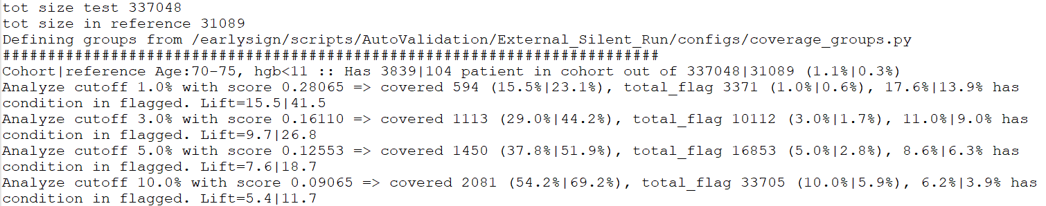
What is actually done? Compare results (reference vs new dataset) in special group, where rate of positive is expected to be high. How to read the results? Important: In the reference, we don't have missing values (-65336), but in the new dataset feature matrix we have. Until fixed, be careful in setting the risk groups. The following is example of results for Test 6 (see 06.coverage.log) First we see that the size of the cohort is small, especially in the reference (just 104 patients). Moreover, the prevalence is much smaller in the reference - 0.3% compared to 1.1%. The difference is high, and probably resulted from the age distribution differences. Next, for every positive rate 1, 3, 5, 10% (numbers below are example for 3%):
- The test calculates cutoff in the tested dataset (0.1611)
- How many flagged? 1113, that are 29% of the cohort (and 11% of the flagged), so lift is 9.7 (29 / 3)
- In the reference, for the same 3% cutoff, just 1.7% would be flagged, including 44.2% of the cohort (who would be 9% of the flagged) => lift of 26.8 (44.2 / 1.7) Conclusions:
- Difference looks significant. Note that the large difference in the the 'lift per cutoff value' is influenced by the difference in incidence rate, but the differences between the tested dataset and the reference are evident from any aspect.
- If the model flag less from this cohort, then, from what cohort it flags more? more investigation is needed before we can come up with applicable lesson.